Life expectancy isn’t what you think

I teach a class on development here at the KDI School. One of the things I like to do is introduce students to different empirical measures of progress we have made in development – especially with respect to poverty – over the past few decades. During a week on human capital, we talk about mortality and life expectancy. We have made huge strides across the globe in reducing child mortality and increasing life expectancy.

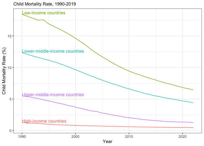
This is easy to see in the data, which I have taken from Our World in Data (Dattani et al. 2023). The data show that child mortality has fallen dramatically over the past few decades. The graph below shows the percentage of children who die before reaching their fifth birthday. Over just forty years, the child mortality rate in low-income countries has decreased from 18.44 percent to 6.45 percent. Wonderful progress, indeed!

But while child mortality is relatively straightforward to interpret, life expectancy is a bit more difficult. I always ask my students what “life expectancy” means. Most of the time, I get a response along the lines of “it is how long we expect someone born today to live.” This, however, is not quite right! Instead, it uses current age-specific mortality rates to calculate the average number of years a person can expect to live if they were to experience the age-specific mortality rates of a given period over the course of their life. What?

Life expectancy with data

Let’s look at some data to put this in context. I have downloaded data from the UK’s Office of National Statistics, which you can find here. Specifically, I have taken the data on male life expectancy in England and copy-pasted that into a new csv file. Let’s load the data and see what it shows.

library(tidyverse)

data <- read_csv("mortalityengland.csv")
data <- data |>
    select(age, mortality=`2021-2023`) 

head(data)

## # A tibble: 6 × 2
##     age mortality
##   <dbl>     <dbl>
## 1     0  0.00455 
## 2     1  0.000244
## 3     2  0.000172
## 4     3  0.000106
## 5     4  0.000084
## 6     5  0.000086

Looking at the data, you can see that at age zero, the mortality value is 0.0045. This means that the probability a child dies before turning one is 0.0045, or 0.45 percent. Another way to think about this is that for every 100,000 children, 455 will die before their first birthday, while 99,545 will survive.

Of those survivors, we can continue to age one, where age-specific mortality is 0.0002. We can do the same calculation, and see that approximately 99,521 children, out of the original 100,000, will survive to their second birthday.[1]

Now, you could imagine going through this process with all 100,000 newborns, calculating the probability of surviving or dying at a given age, using these age-specific mortality rates. We could make sure to note the age at which a hypothetical person dies, and then using this age for our 100,000 people, calculate the average age at death. This is exactly what life expectancy is: it is the average age at death using current age-specific mortality rates.

Let’s do that with the data. First, a small note: the data I downloaded stops at age 100. We are going to assume anyone still alive at 100 dies then. This means that our life expectancy calculation will be slightly low, but it should still give you a good idea of how this works. Let’s make that change at age 100:

# assume everyone dies at 100
data$mortality[data$age==100] <- 1

Now, we are going to calculate the probability of surviving at each age, for 100,000 different people. We will do this using one of R’s most powerful tools: apply functions. When I first learned R, I avoided these and defaulted to for loops, which is what I was use to. But the apply functions are much faster and more efficient. We can do this in one line of code:

# get 100,000 people, randomly draw values
set.seed(130945)
random_samples <- sapply(data$mortality, function(x) sample(0:1, 100000, prob=c(1-x, x), replace = TRUE))

Let me explain these two lines of code. The first line is setting a seed. This allows us to reproduce a (pseudo) random function in R. The second line usins the sapply() function, and we tell it to go through every single value of data$mortality. For each value, we sample 100,000 values from a binomial distribution, where the probability of success is 1 - data$mortality. This means that if the mortality rate is 0.01, the probability of surviving is 0.99. So, for each person, we get a probability of surviving at each and every age. The new random_samples object will have dimensions of 100,000 x 101, where each row is a person and each column is an age (from 0 to 100, so 101 values).

Now this doesn’t quite get us to where we want to go. What we are going to do is find the first time an individual “dies” – that is, the first time they have a value of 1. We can then use which() to find the age at which they die:

death_events <- apply(random_samples, 1, function(sample) {
    which(sample == 1)[1]
})
death_events <- death_events - 1
mean(death_events)

## [1] 78.60119

We are again using one of the apply functions, this time apply(). We are telling apply() to go through each row of random_samples (that is what the 1 represents; if you wanted to go through columns, you would use a 2 instead), and for each row, find the first time they have a value of 1, which in our example represents mortality.[2] Since the first value is actually age zero, we then subtract one from the result. Finally, we take the average of all these ages, which gives us the average age at death.

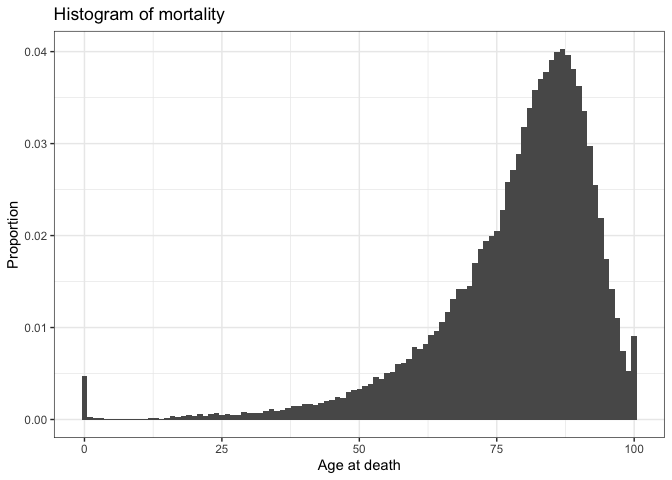
We can plot this using a histogram, with 101 bins (one for each age):

ggplot() +
    geom_histogram(aes(x=death_events, y=after_stat(count/sum(count))), bins=101) +
    labs(title="Histogram of mortality", x="Age at death", y="Proportion") +
    theme_bw()

There you have it! This shows the distribution of ages at death, using the age-specific mortality rates for 2021-2023 England. By taking the mean across all these ages, we get the average age at death, which is 78.6 years. This is a slight underestimate of the official value, which is most likely due to the fact that we assumed everyone dies at age 100. Indeed, we can see the increase in mortality at age 100 in the histogram above; many of them would have lived to be older, but we cut them off at 100 since we didn’t have data beyond that age.

References

Dattani, Saloni, Fiona Spooner, Hannah Ritchie, and Max Roser. 2023. “Child and Infant Mortality.” Our World in Data.

[1] It’s worth noting that mortality rates for children are quite high just after birth, but then decrease rapidly. This is why the number of survivors is so high at age one relative to age zero.

[2] which(sample == 1) returns the index for ALL values of 1, but we just want to extract the first value, which we do with the [1] at the end.